Library › Calculating AI by Hand ✍️
Support Vector Machines (SVMs) reigned supreme in machine learning before the deep learning revolution.
In every model so far, both the forward and backward passes are matrix multiplications, which is exactly what GPUs accelerate. An SVM is different: its prediction is still built on matrix multiplication (dot products between vectors), but it is trained by convex optimization rather than backpropagation, so there is no matrix-multiplication backward pass to hand to a GPU. That is a big reason SVMs never rode the GPU and big-data wave that powered deep learning.
I took great effort to lay out this SVM exactly like an MLP, using the same matrix-multiplication format, so you can visually compare and see how similar the prediction step looks.
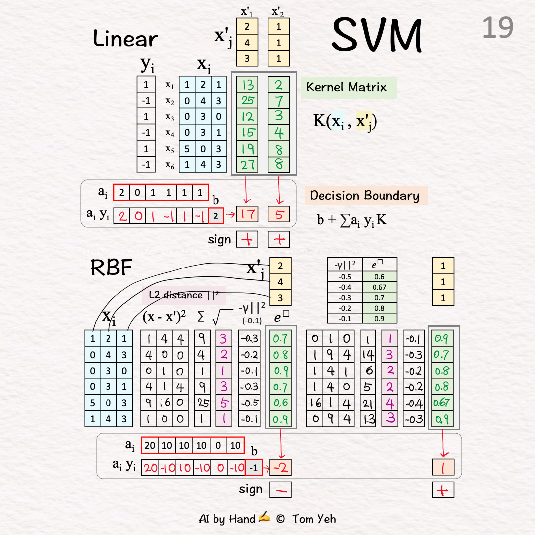
This exercise compares Linear and RBF SVMs: how each classifies two test vectors, using support vectors learned from six training vectors.

Setup
Step 1 of 19: Given
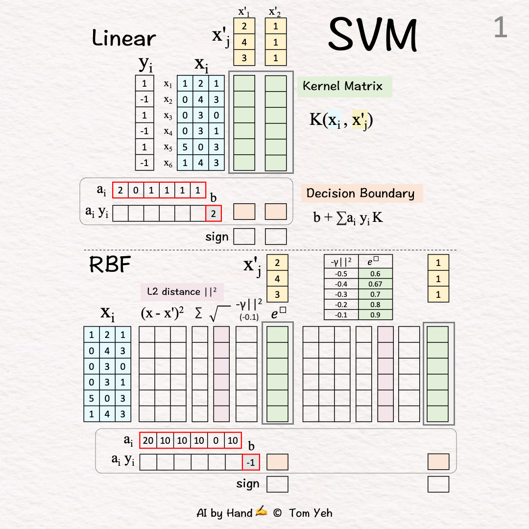
xi: Six training vectors (blue rows 🟦) yi: Labels
Using xi and yi, we learned ai and b (red borders):
ai: coefficient for each training vector i.
Non-zero: A Support Vector that defines the decision boundary
Zero: Too far from the decision boundary, ignored
b: bias (how much the decision boundary should be shifted)
x’j: Two test vectors (yellow columns 🟨)
(To simplify hand calculation, training and test vectors are not normalized.)
Linear SVM
Kernel Matrix
Step 2 of 19: Test Vector 1
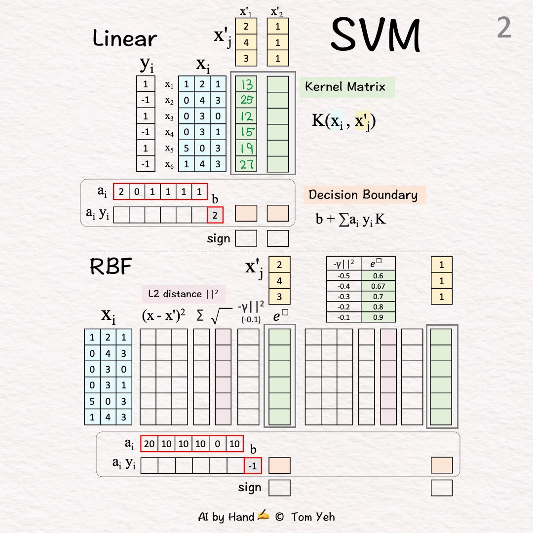
Take dot product between the test vector 🟨 and every training vector 🟦
The dot product approximates the “cosine similarity” between two vectors
Output: 1st column of K
Step 3 of 19: Test Vector 2
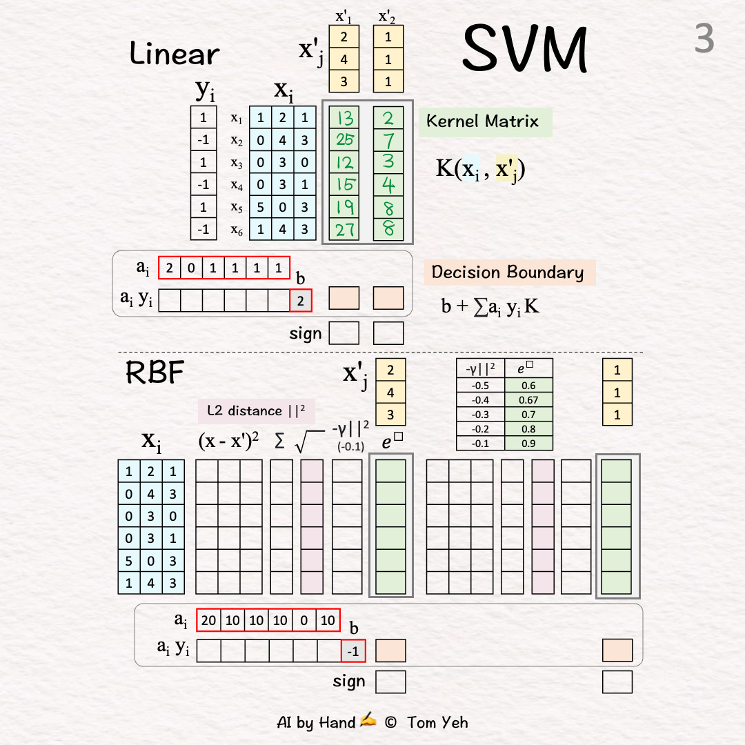
Similar to [2]
Output: 2nd column of K
Decision Boundary
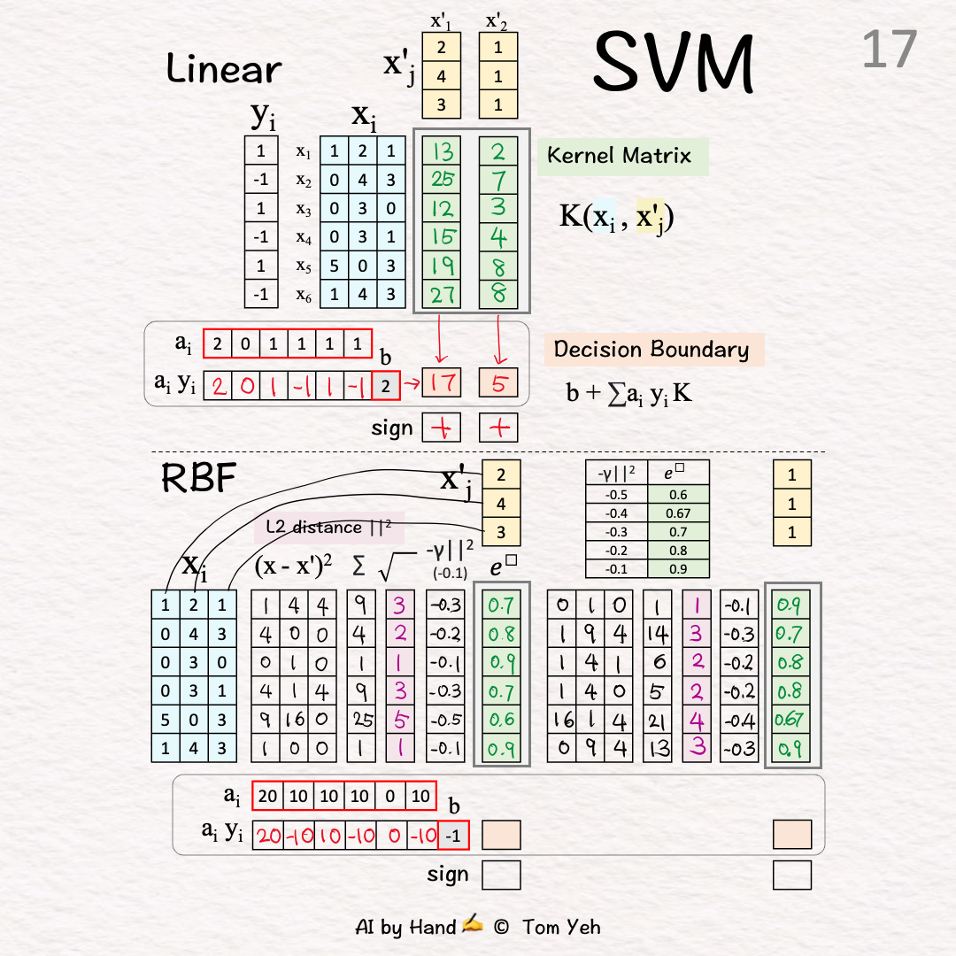
Step 4 of 19: Signed Weights
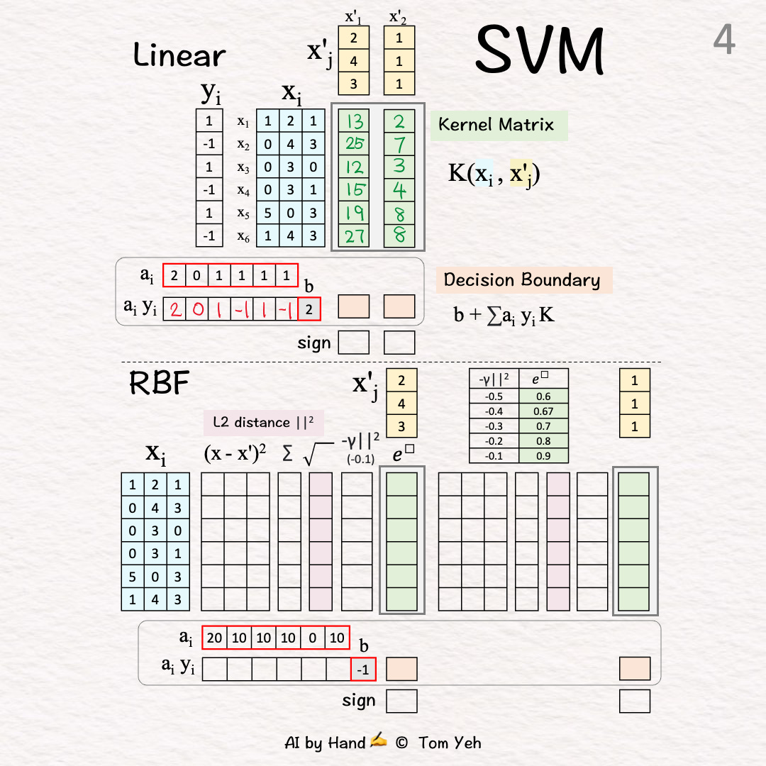
Multiply each coefficient with the corresponding label
The 2nd training vector is NOT a support vector because its coefficient is 0.
Step 5 of 19: Weighted Combination
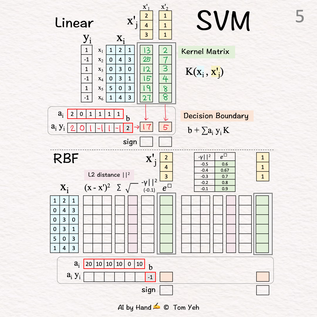
Multiply weights and bias with K
Output: “signed” distance to the decision boundary
Step 6 of 19: Classify
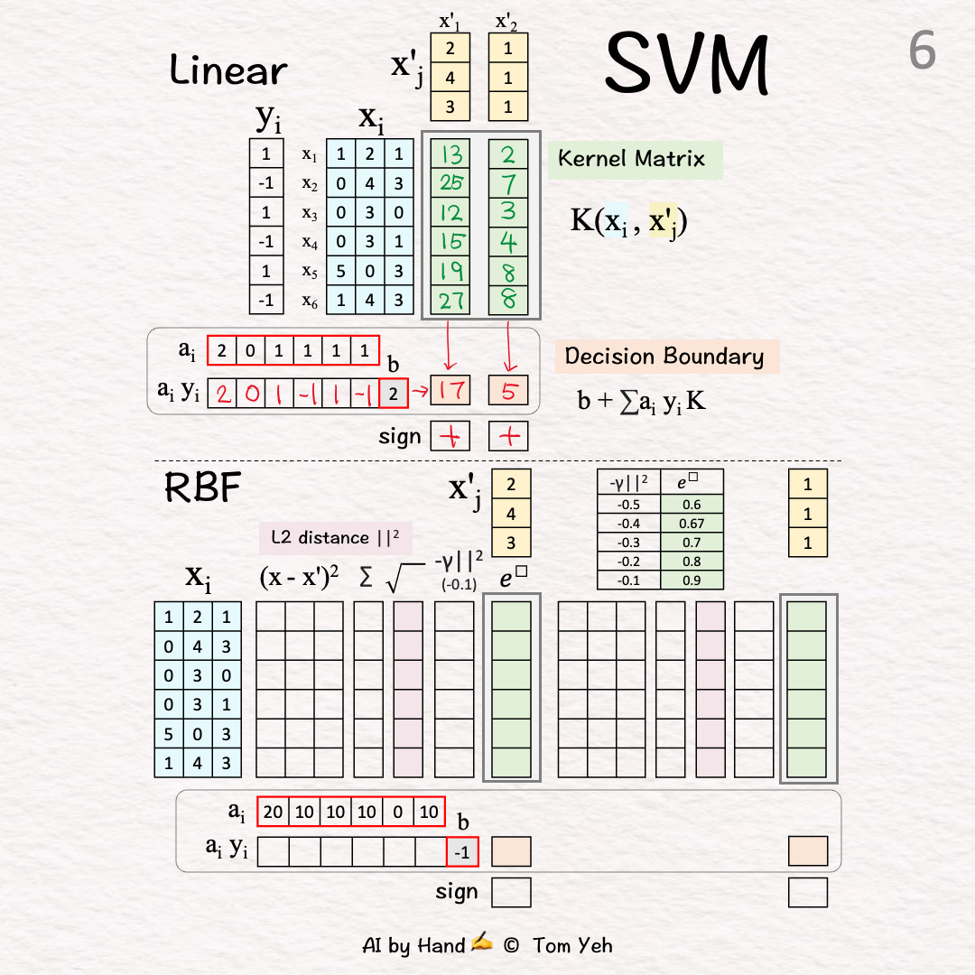
Take the sign
RBF SVM
Given ai: Learned coefficients b: Learned bias
Kernel Matrix
Test Vector 1
L2 Distance
Step 7 of 19: Squared Difference
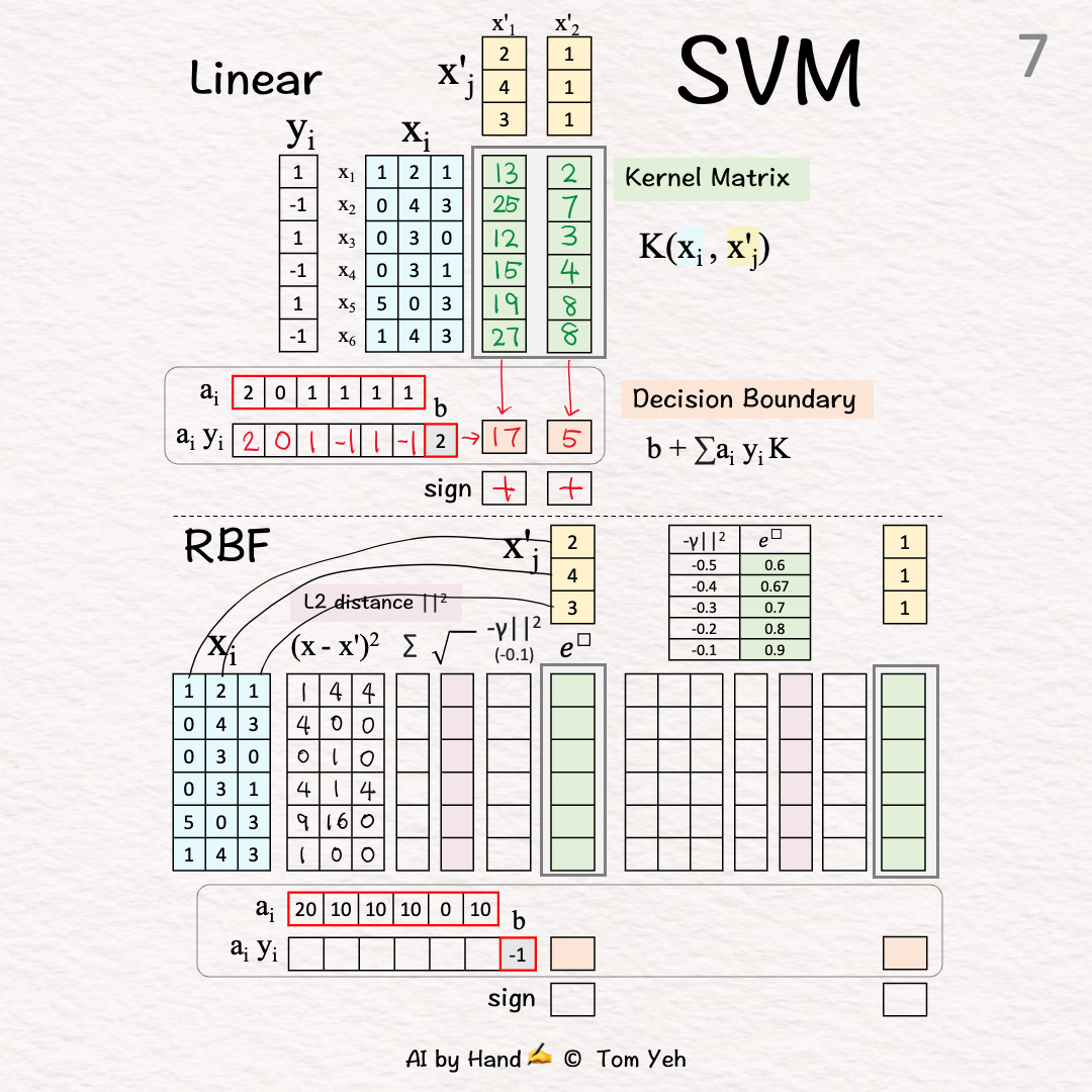
i=1: (1-2)^2=1, (2-4)^2=4, (1-3)^2=4
Step 8 of 19: Sum
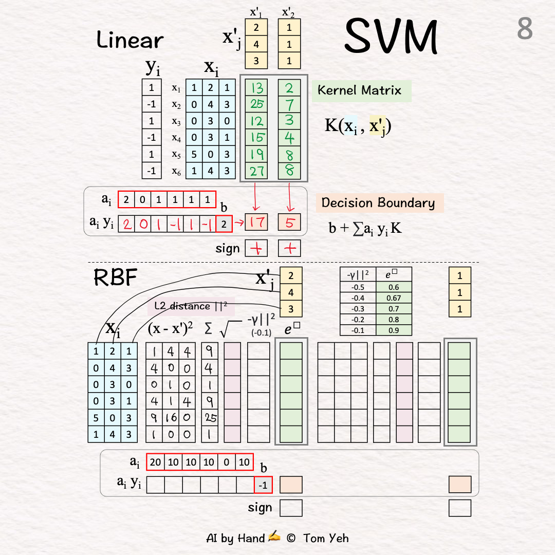
Step 9 of 19: Square Root
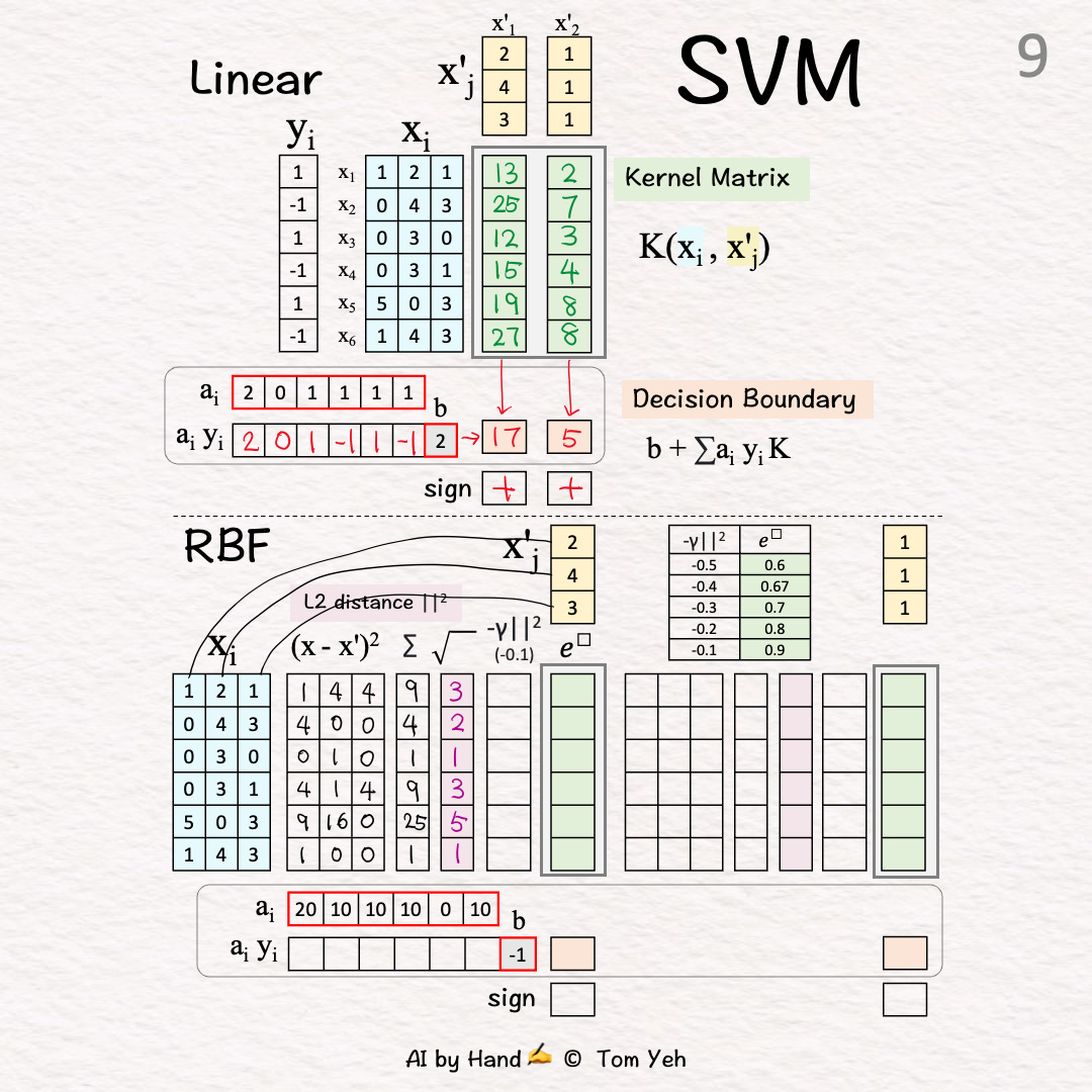
Step 10 of 19: Negative Scaling
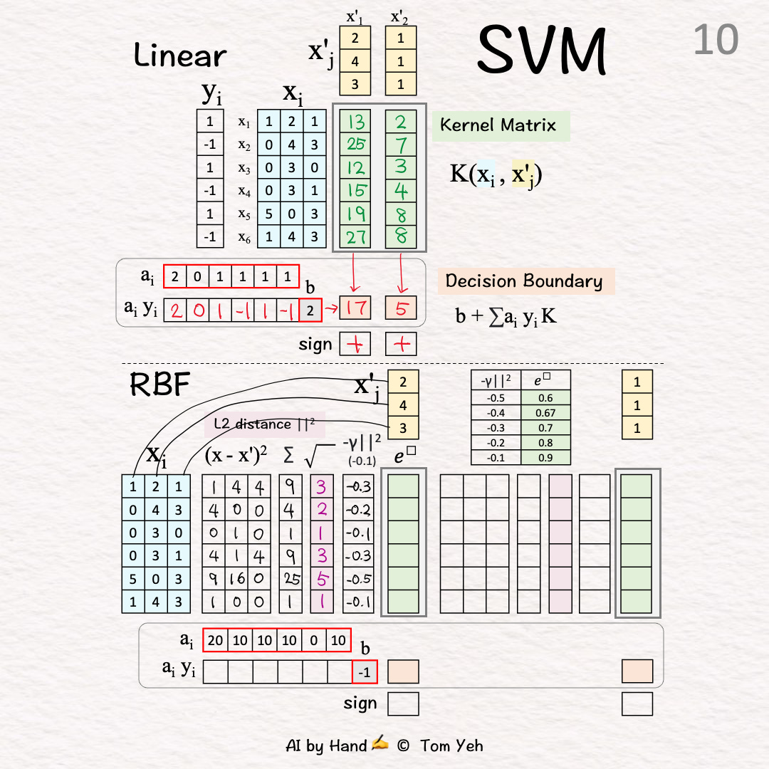
Multiply by -1: Note that L2 is a distance metric. The negation converts distance to similarity.
Multiply by gamma γ: The purpose is to control how much influence each training example has. A small gamma means each training example pulls the decision boundary more lightly, resulting in smoother decision boundaries.
The result is “negative scaled L2”
Step 11 of 19: Exponentiate
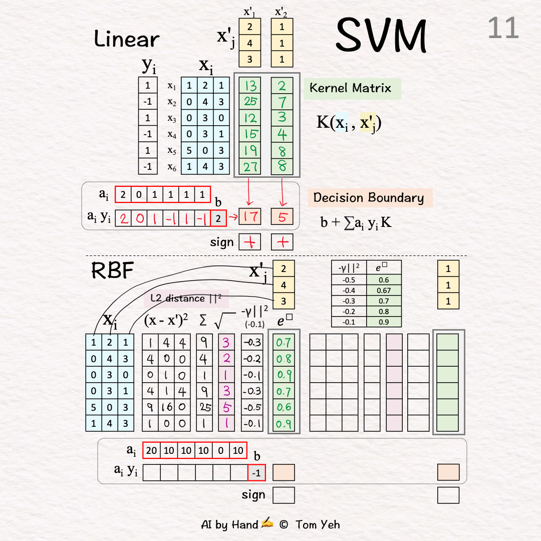
Raise e to the power of the “negative scaled L2”
Use the provided table to look up the value of e^
Output: The 1st column of K
Test Vector 2
L2 Distance
Step 12 of 19: Squared Difference
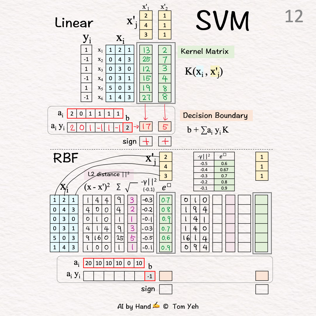
Step 13 of 19: Sum
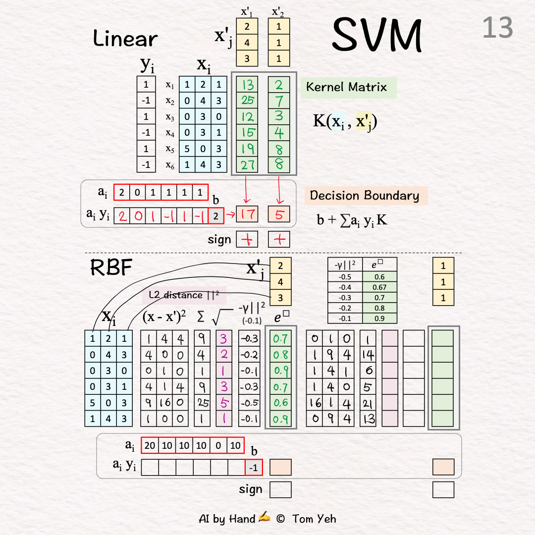
Step 14 of 19: Square Root
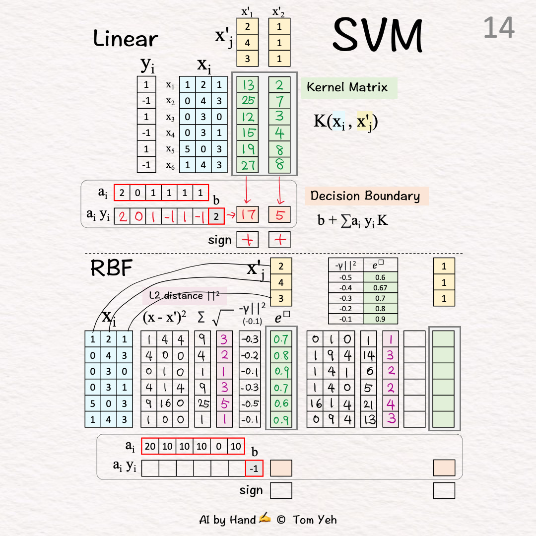
Step 15 of 19: Negative Scaling
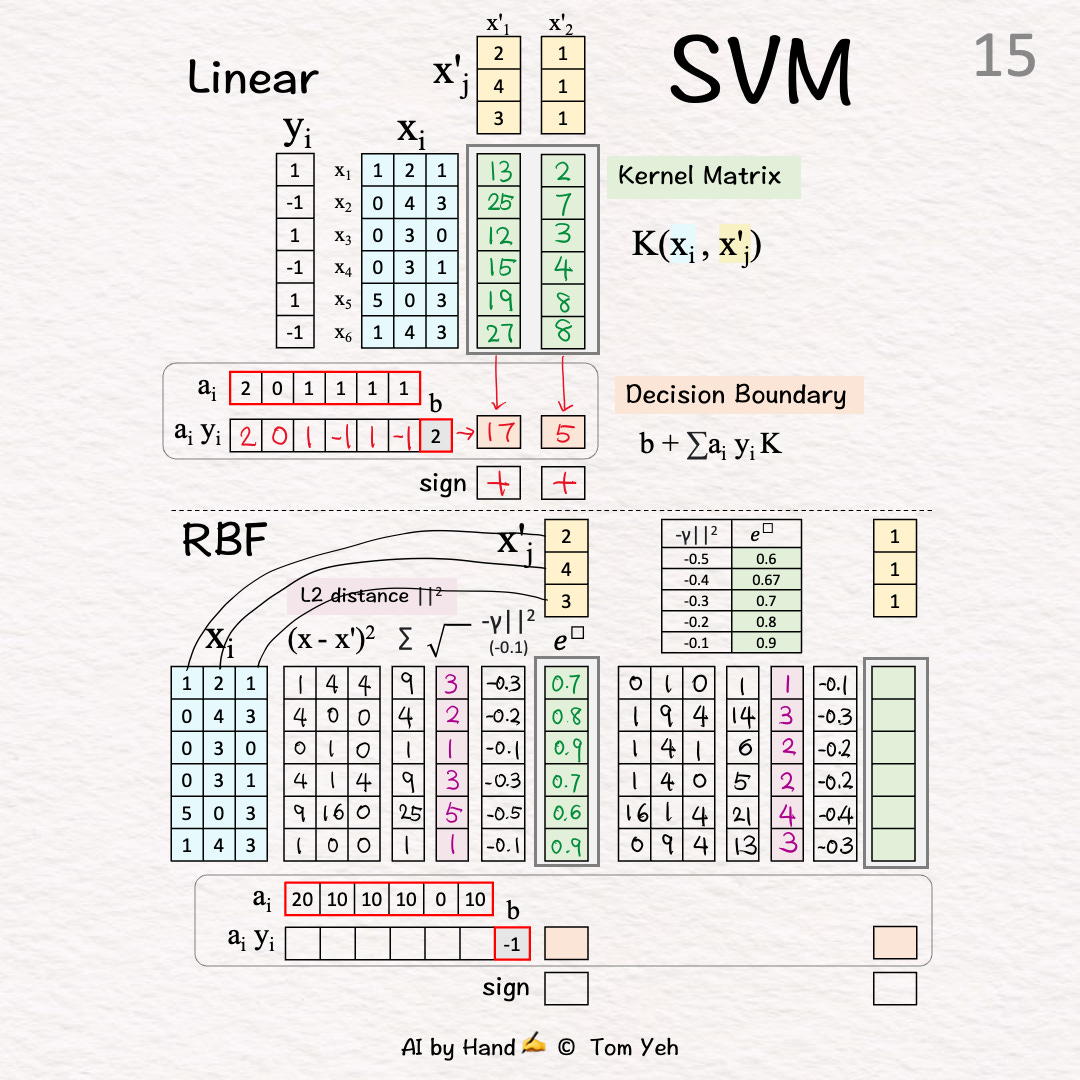
Step 16 of 19: Exponentiate
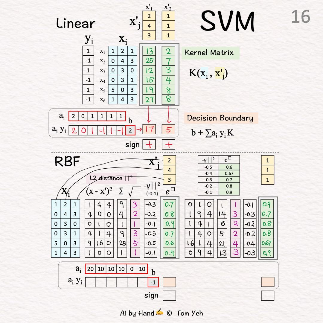
Output: The 2nd column of K
Decision Boundary
Step 17 of 19: Signed Weights
Step 18 of 19: Weighted Combination
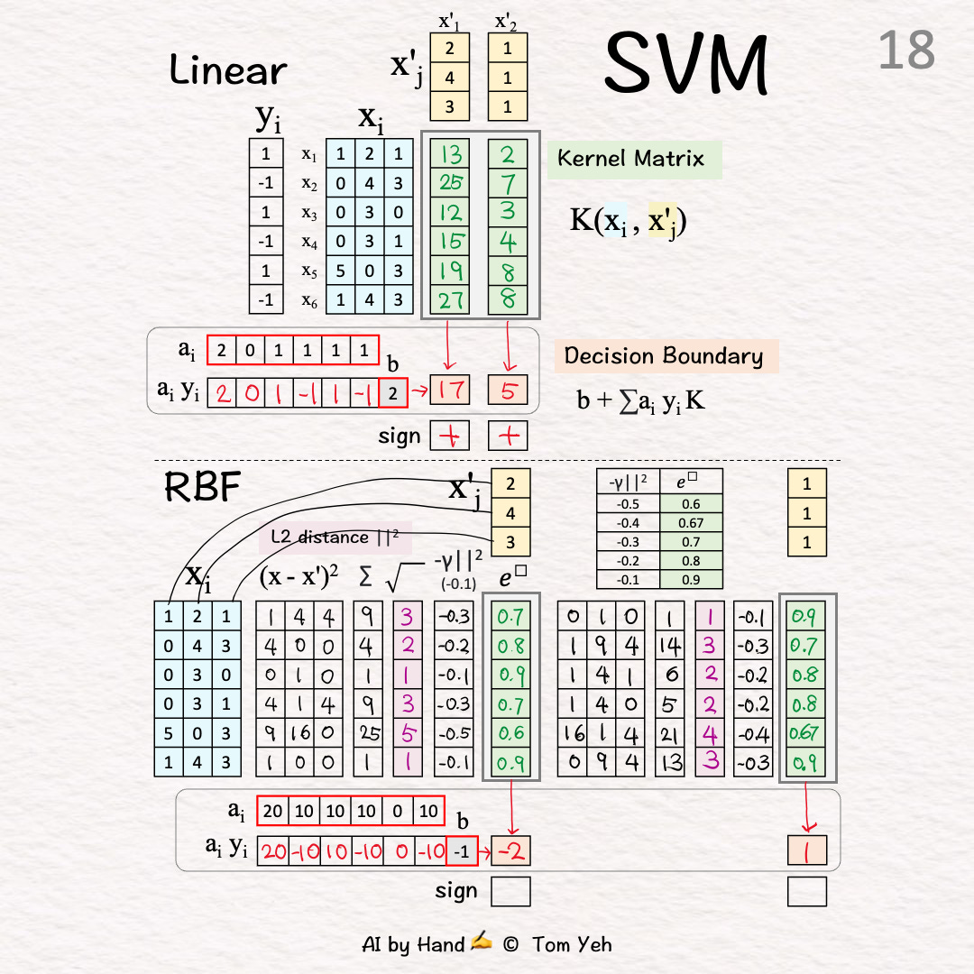
Step 19 of 19: Classify